Risk-based UAS Trajectory Optimization

Case Study

Commercial drone operators, or those managing unmanned aerial systems (UAS), are obligated to comply with CR14 Part 107 regulations to operate drones and maintain certification, which presents planning challenges due to airspace restrictions, weather conditions, midair collision, and other factors. Severity is influenced by factors such as population density under planned flight paths, impacting the risk of human casualties.

In light of these risks, finding a safe, regulated, and short trajectory for a UAS becomes a complex optimization problem. Quantum Computing Inc (QCi) uses realistic data from our partner, ATA LLC - a data science company and Low Altitude Authorization and Notification Capability (LAANC) service provider, to construct two models: one algorithmically solvable and the other NP-complete, indicating an absence of polynomial-time solutions as the problem size increases. We demonstrate the efficiency of a hybrid quantum optimization machine, an Entropy Quantum Computing (EQC) system called Dirac-1 in solution quality and time scalability.

Method

The nature of this problem is a decision problem that answers the question: Which trajectory should be taken to minimize risk when leaving point A and arriving at point B?

Decision Model

The model chosen to represent the decision has two main criteria. The first criterion is to answer the question of the decision problem. Secondly, it is necessary to ensure a drone has the capacity to fly the planned trajectory. Satisfying these two goals with the same solution gives the necessary result to model a desired trajectory plan. We will refer to the model that only answers the decision question without time as LR for `Lowest Risk`. The second model, which ensures timeliness, will be referred to as LRTC for `Lowest Risk with Time Constraint`.

The simpler model, LR, can be solved using an existing polynomial algorithm (Dijkstra's algorithm). We have many options for fast classical computing implementations of Dijkstra's algorithm to solve the first model. In fact, many enhancements have been made for special cases, but the worst-case performance on fully dense graphs is still no better than $O(n^2)$ $O (n^{2})$ , which was from Edsger Dijkstra in 1959. This worst-case performance doesn't call for quantum, even with very large graph structures. With modern computing power, the examples here take only milliseconds to solve.

However, the LRTC, which adds the time constraint, puts this problem into the set of NP-hard problems, which cannot be addressed with traditional graph shortest path algorithms. It is known that this model is NP-complete, although weakly NP-complete as Cai, Kloks, and Wong, also Yang, Gao, Yu, and Li have described pseudo-polynomial algorithms for this problem and variants. Shortest path with time constraints is now interesting from a computational perspective and worthy to explore using alternative computing methods.

Formulating the Problem

Risk can be computed by using a cost function of expected loss. Expectation of risk from this perspective is cost multiplied by likelihood. It is easy to see how this can be utilized to avoid routes that have a higher likelihood of events such as human casualty: simply increase the cost to a level sufficient that discourages those choices. This is simple in concept, but in practice can be challenging because of numerical (classical) and dynamic range (quantum) issues it can cause. Instead, values only sufficiently high should be used with this modeling choice. The levels, risk score, and edge weight values are listed in Table 1. The risk score values come from the ATA Beeline application. These risk score values are directly translated into risk weights for our graph data structures using this formula which is parameterized to have the lowest weight as 1: $w = 2^{10x-3}$ $w = 2^{10 x - 3}$ where $w$ $w$ is the weight and $x$ $x$ is the risk score.

Risk Level	Risk Score Risk	Weight
Manageable	0.3	1
Major	0.6	8
Hazardous	0.8	32
Catastrophic	1.0	256

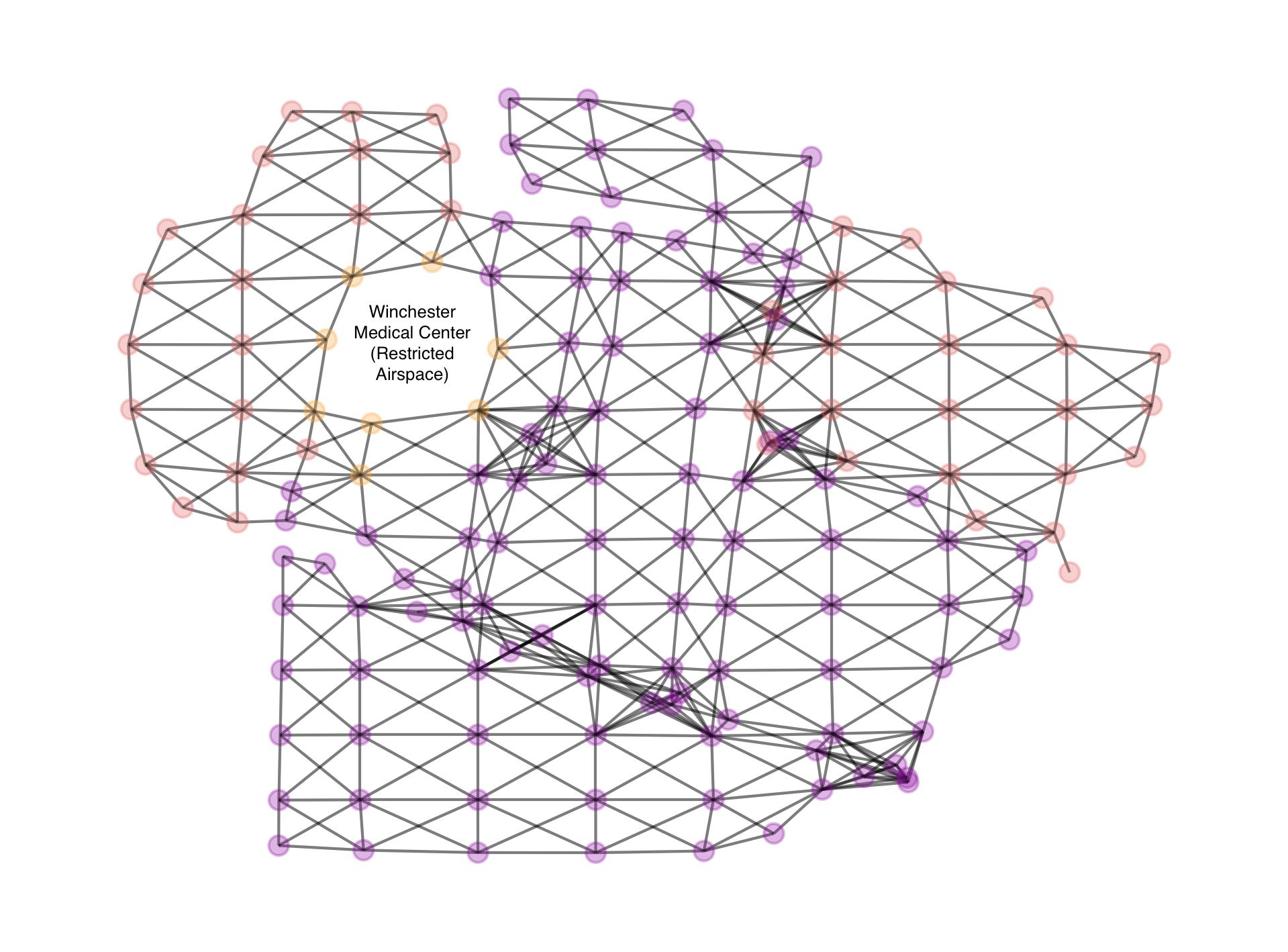
The two flight trajectory criteria chosen for the model are incorporated into mathematical terms using graph theory and integer programming. First, we take the map segments with associated risk provided by ATA and represent them using nodes and edges. The general layout of the map segments is a Cartesian grid, but partial segments may be included in a map if the bounding polygon cut off part of each segment. The edges are given the weights associated with the appropriate level of risk. See figure 1 for a visual representation of the graph for one map. This graph is undirected, but in practice, a directed graph with two edges between each pair of nodes is used. The graph is built by determining the segments that intersect with each other, even if at only a single point, then adding each segment as a node with two edges between each pair of intersecting nodes.

winmed graph — Graph representation of a flight region

The graph representation of a map is useful in many contexts and provides a good starting point for mathematical models.

Edge Weights

Each map segment is represented by a node in the graph, and each node carries a corresponding risk weight. However, risk weights must be assigned to the graph edges, each of which connects two nodes. This presents a question of how to choose which risk weight to assign to each edge weight. Three alternatives seem most obvious.

item Use the risk weight of the leaving node,
item use the risk weight of the entering node, or
item use the average risk weights of the leaving and entering nodes.

The first and second alternatives would have the effect of counting the full risk of either the starting or ending node and not the other, while the third alternative would count half the risk of each of the starting and ending nodes. Although these should all result in the same route choices, the third alternative was chosen since it allows a single value to be used on each of the directed edges between the two nodes whereas the other two options require different values depending on the direction of the edge.

Distance, Time, and Speed

Map segments are defined by projections of the earth's surface onto polygons. Most of these polygons have a single height and width, and thus are rectangles. Some polygons are not regular because of the selection used to define a particular flight region. Also, the height and width are not as important as the point used to represent each polygon. The polygon centroids determine the Cartesian coordinates of each node. Distances between the centroids of adjacent map segments are measured and used to determine time to traverse from one node to another.

Mathematical Description

Term	Description
$G(V, E)$	graph representation with nodes in $V$ $V$ and edges $E$ $E$
$t_{ij} ∈ R$	time to traverse from node $i ∈ E$ $i \in E$ to node $j ∈ E$ $j \in E$
$r ∈ R$	assumed average speed of a UAS in meters per second
$T ∈ R$	maximum time allowed for flight trajectory in seconds
$s ∈ E$	starting node in a request
$t ∈ E$	ending node in a request
$x_{ij} ∈ \{0, 1\}$	Binary variable indicating the traversal from node $i$ $i$ to node $j$ $j$
$w_{ij} ∈ \{1, 8, 32, 256\}$	Risk weight for traversing from node $i$ $i$ to $j$ $j$

The risk-optimal model is exactly a shortest path model integer programming (IP) formulation with special consideration given to the weights. Each node has a constraint associated which indicates whether it must be balanced (a leaving edge for every arriving edge) or must have one more leaving edge or arriving edge than the other in the cases of the start and end nodes, respectively. The minimization objective keeps superfluous edges from forming cycles, which would still satisfy the constraints. The IP formulation using the terms in Table 2 is

\quad\quad\min_x \, \sum_{(i,j) \in E} w_{ij} x_{ij}\quad x\in \{0, 1\}

\mathrm{s.t.}\quad\quad\quad \sum_{j}x_{ij} - \sum_{j}x_{ji} = \begin{cases} 1 & \mathrm{ if }\, i=s \\ -1 & \mathrm{ if } \, i=t \\ 0 & \mathrm { otherwise} \end{cases} \quad \forall i \in V

Adding a single constraint to the risk-optimal model results in the time constrained risk-optimal model. That constraint is

$\sum_{(i,j)\in E} t_{ij}x_{ij} \leq T$ $\sum_{(i, j) \in E} t_{ij} x_{ij} \leq T$

which means the sum of the times ( $t_{ij}$ $t_{ij}$ ) it takes to traverse selected edges ( $x_{ij}=1$ $x_{ij} = 1$ ) is less than or equal to the time constraint, $T$ $T$ . This constraint is known as a knapsack constraint.

Time Constraint

The time constraint requires some simple calculation for input into the model. In all cases, we have assumed an average UAS flight speed of 7 meters per second. For each edge, the time to traverse this edge is calculated by finding the approximate distance between the centroids of the polygons the nodes represent by calculating the Haversine distance using a radius of 6,369,345 m. This is translated into seconds by dividing the approximate distance by the speed, 7 m/s.

Maps

We have four maps to analyze with unique risk profiles. A selection of 100 random pairs of segments is chosen from each map for the start and end points of trajectories to find. Some of the points randomly selected result in problems which are infeasible, even without the time constraint, so the number of problems may be slightly lower than 100. These four maps are around the towns of Winchester and Yorktown VA. See Table 3 for a listing of the maps. Each map has a range of risk listed in the table. The nodes and edges listed in the table show the size of the graph generated for each map. It should be noted that LR has a variable count equal to the number of edges. LRTC has an additional set of auxiliary variables to translate the inequality constraint to equality. For the constraint, we have used a max time of $T=600$ $T = 600$ seconds, which requires 10 binary variables to encode, so in general, there are 10 more variables than edges.

Map Name	Nodes	Edges	Minimum Risk	Maximum Risk
winchester_001	159	1156	Manageable	Hazardous
winchester_003	26	128	Manageable	Hazardous
yorktown_002	87	1066	Major	Hazardous
yorktown_003	100	754	Major	Catastrophic

After obtaining a solution by any of these methods, a map of the trajectory can be generated. Each map includes the grid segments that have risk calculated. The color legend of the risk levels is in figure 2.

Solver Choice

We explore two different solvers for this problem including

item NetworkX shortest_path - a Python package with an implementation of Dijkstra`s algorithm
item QCi Dirac-1 entropy quantum computing system - hybrid quantum machine for solving binary optimization problems.

Table 4 shows which models can be compared across solvers/devices. Solutions to this problem are obtained in two stages. The first stage is performed using Dijkstra's algorithm. The solution obtained from this stage is tested for the time requirement. If the time requirement is less than or equal to the max time allowed, then the second stage is not necessary. The second stage is to solve LRTC. This stage builds an integer formulation and translates that into a QUBO. The method of translating the IP model into a QUBO is well-known. This QUBO is sent to the QCi Qatalyst\texttrademark \ API to be solved by Dirac-1. A solution to LRTC will have a risk score no better than the risk score obtained by solving LR, but it will meet the time constraint, if possible. This means that solutions to LRTC will still minimize the risk, but while keeping the flight trajectory feasible.

Solver	LR	LRTC
NetworkX (Dijkstra)	X
Dirac-1	X	X

Results

Algorithmically Tractable

Results from the first stage which the LR model was solved using an algorithm with a polynomial time scale are reported here. NetworkX provided clear results of trajectories that avoid risk in a computationally efficient manner. Figure 2 illustrates an example of the optimal route result for the Winchester Medical Center case. This route is over the time allowed by 19 seconds. A solution to the model must be interpreted exactly to allow for input which creates cushioned values, so 19 seconds over the time limit is reason enough to find an alternate.

winmed nx final color — Risk-optimal solution to Winchester Medical Center case in LR model

Table 5 summarizes the results of solving using the LR model on four different maps. It can be seen that all solutions are not satisfied with the maximum allowed time.

NP-complete

We solve this problem by applying the LRTC model, making this optimization problem NP-complete. Dirac-1 produces a trajectory that honors the time constraint and also minimizes the risk. This trajectory visits 6 major risk nodes and one manageable risk node, giving a risk score of 49. This is higher than the risk-optimal route, which visits only a single node of major risk severity. Presented with this information, a pilot could make the determination of whether or not to fly the route.

Map Name	Trajectories	Infeasible Trajectories	LR Results within Max Time
winchester_001	100	46	54.0%
winchester_003	98	89	9.2%
yorktown_002	98	74	25.4%
yorktown_003	97	62	36.1%

Table 5: Summary of optimal trajectories found using NetworkX on LR model. Results exceed the maximum allowed time, indicating the need for a time-constrained model

winmed eqc final color — Solution returned by Dirac-1 to Winchester Medical Center case satisfied the time constraint while minimizing the risk

Figure 3: Solution returned by Dirac-1 to Winchester Medical Center case satisfied the time constraint while minimizing the risk

Model	Solver	Risk Objective	Trajectory Duration	Honor Time Constraint
LR	NetworkX	14	10 minutes 19 seconds	N
LRTC	Dirac-1	49	7 minutes 6 seconds	Y

Table 6: Summary of typical results for Winchester Medical Center case using an algorithmically solvable model with NetworkX and an NP-complete model on Dirac-1

Scalability

Here we study the scalability of Dirac-1 where we run the same models with an increasing number of variables to observe the time-to-solution trend. We have generated a new map instance that is derived from the winchester\_003 map by dividing segments into four parts recursively. The four parts are created with two orthogonal dividing lines crossing at the centroid of the segment. This method allows us to test the model above 10,000 variables.

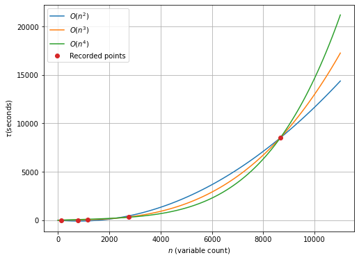
At 10,364 variables, this instance was run on Dirac-1 five times and returned the average of 13,852 seconds per solve. Figure 4 shows some insight into time performance as a direct comparison to computational complexity for time. Polynomials of order 2, 3, and 4 originating at the origin, (0, 0), were fit through the data points and plotted. Each polynomial takes the form: $y = c_1 n^p + c_2 n$ $y = c_{1} n^{p} + c_{2} n$ to capture the possibility of higher degree growth in time to solution, but not over fit the data and result in multiple points of inflection.

This fits between the $n^2$ $n^{2}$ and $n^3$ $n^{3}$ performance scale models, indicating that Dirac-1 scales performance better than $O(n^3)$ $O (n^{3})$ ) along some approximate function $c_1n^2+c_2n + M$ $c_{1} n^{2} + c_{2} n + M$ where $c_1$ $c_{1}$ , $c_2$ $c_{2}$ , and $M$ $M$ are constants.

performance prediction — Time-to-solution on Dirac-1 vs. problem size of the LRTC model on one map. Fitting curve follows second, third, and fourth-order polynomials showing that Dirac-1 does not explode in time-to-solution on an NP-complete problem

Conclusion

We have demonstrated the application of the QCi Dirac-1 entropy quantum computing system to solve an NP-complete/NP-hard, time-constrained risk-based trajectory selection problem for unmanned aerial systems.

While the solutions provided by NetworkX for the LR model may find the lowest risk trajectories, the model that NetworkX is capable of solving ignores the real-world constraint that UAS drones have limited flight time capacities. Thus, there is an inherent need for the second and more sophisticated LRTC. Since LR has performance guarantees for any conceivable problem size, it could be used until it provides a result that does not meet the UAS limitation on flight time. The LRTC model provides a superior solution to the problem, but is NP-complete, making conventional computing methods less capable of finding good solutions for it as the problem size grows. Dirac-1 was able to solve this NP-complete problem within polynomial time, even at large scale- more than 10,000 variables. This promises great potential as an alternative computing method for operational optimization.

Future Works

While the time-to-solution of Dirac-1 correlates with problem size following a polynomial curve, it is crucial to minimize the coefficient amplitudes of this curve. We will continue to improve the results of this case study using Dirac-3. QCi is dedicated to enhancing this aspect further by transitioning the hybrid quantum optics and digital electronics to most-optical and all-optical systems. This move aims to fully leverage the speed of light and quantum parallelism computation.

References

Ravindra K. Ahuja, Thomas L. Magnanti, and James B. Orlin. Network Flows: Theory, Algorithms and Applications. 1st. Pearson, 1993.
[2] X. Cai, T. Kloks, and C. K. Wong. “Shortest path problems with time constraints”. In: Mathematical Foundations of Computer Science 1996. Ed. by Wojciech Penczek and Andrzej Szałas. Berlin, Heidelberg: Springer Berlin Heidelberg, 1996, pp. 255–266. ISBN: 978-3-540-70597-0.
[3] Certified Remote Pilots including Commercial Operators. URL: https://www.faa.gov/uas/commercial_operators. (accessed: 12.12.2022).
[4] Guide to the Instance Statistics. URL: https://miplib.zib.de/statistics.html. (accessed: 1.22.2023).
[5] Aric A. Hagberg, Daniel A. Schult, and Pieter J. Swart. “Exploring Network Structure, Dynamics, and Function using NetworkX”. In: Proceedings of the 7th Python in Science Conference. Ed. by Gaël Varoquaux, Travis Vaught, and Jarrod Millman. Pasadena, CA USA, 2008, pp. 11–15.
[6] Yajun Yang et al. “Finding the Cost-Optimal Path with Time Constraint over Time-Dependent Graphs”. In: Proc. VLDB Endow. 7.9 (May 2014), pp. 673–684. ISSN: 2150-8097. DOI: 10.14778/2732939.2732941. URL: https://doi.org/10.14778/2732939.2732941. 11