Default
Dirac Quick Start
Welcome to the Quantum Computing Inc. (QCi) quick-start guide for cloud-based Dirac computing devices! This page walks you through accessing our quantum optimization devices, including Dirac-1 and Dirac-3. While these devices can be accessed in your preferred programming language via a REST API, the qci-client package wraps the API's HTTP calls in Python methods to remove the requirement of knowing how to perform HTTP interactions. Either way, an access token is required for the API, and one can be requested below. Following the receipt of an access token, this tutorial shows how to configure your environment for the examples in the Resource Library. The final section covers how to run a simple problem in Python with qci-client. Let's get started!
Obtaining an Access Token
To access our quantum optimization machines and run jobs using the qci-client, you'll need an active account and an API access token.
Once you have your API token, follow the steps below to connect to the qci-client and access our cloud-based devices:
Installation
To follow our tutorial, ensure you have a Python version >=3.9 and <3.14 installed on your system. To install the latest qci-client package run the following command in your terminal:
- pip install --upgrade "qci-client>=4"
This will install the latest version of the qci-client package (version 4 or higher). For a more organized development environment, we recommend using a Python virtual environment to isolate qci-client dependencies.
Configure Environment Variables
Next, setup two environment variables: one for the API's URL and one for your token. The API URL tells the client where to connect, and your API token is what allows you to access the API. The operating system you are using determines how you should configure environment variables. On Linux, MacOS and other UNIX-like operating systems, you can edit the configuration file appropriate for your shell. For .bash_profile or .zprofile, for instance, add these lines (Replace <your_secret_token> with your actual API token, a long string of letters and numbers):
- export QCI_API_URL=https://api.qci-prod.com
- export QCI_TOKEN=<your secret token>
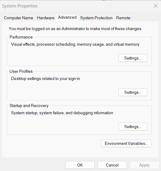
For Windows, you must open System Properties and press the Environment Variables... button on the Advanced tab.
In the Environment Variables window, click New... in the User variables for <your name> pane.
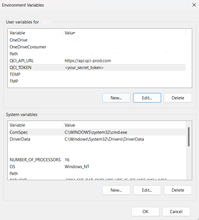
Create the QCI_API_URL and QCI_TOKEN variables with appropriate values.
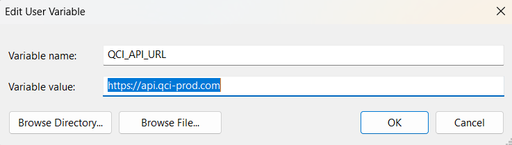
Once both of these variables are created, restart your shell or application such as VS Code to load the new configuration.
Testing Your Setup
Import the qci-client package
- import qci_client as qc
Create a client instance
- # the following line shows how to directly configure QCIClient with variables
- # client = qc.QciClient(api_token=<your_secret_token>, url="https://api.qci-prod.com")
- # if you have configured your environment correctly, the following line should work
- client = qc.QciClient()
This line creates a QciClient object, which acts as your interface to the QCi API. The following statement verifies your token is working correctly and prints the time allocation balance.
- print(client.get_allocations()["allocations"]["dirac"])
Running a small job
Now that we've created a client instance and gained access to the API, let's proceed with running a small optimization problem on our Dirac-3 device. This exercise will us become acquainted with the job pipeline.
First, we'll define the problem we want to solve. We aim to minimize the energy of a Hamiltonian function, which is described by a polynomial in two variables.
The optimization problem
We solve the following problem:
Step 1: Encode the problem data into a JSON file format so that it is recognized by the API. In this step, we prepare example data representing a small problem aimed at minimizing the polynomial:
- # Here we load some example data which represents a very small problem to minimize the
- # polynomial H = -x_1^2 + 2*x_1*x_2 - x_2^2, subject to x_1 + x_2 = 1, x_1>=0, x_2>=0.
- poly_indices = [[1, 1], [1, 2], [2, 2]]
- poly_coefficients = [-1, 2, -1]
- data = [{"idx": idx, "val": val} for idx, val in zip(poly_indices, poly_coefficients)]
- file = {
- "file_name": "hello-world",
- "file_config": {
- "polynomial": {
- "num_variables": 2,
- "min_degree": 2,
- "max_degree": 2,
- "data": data,
- }
- }
- }
Step 2: Upload the JSON file to the API. A unique file identifier (file_id) will be returned in the file_response, allowing for easy referencing of the uploaded data in subsequent tasks. This is useful when running a parameter sweep, for instance.
- file_response = client.upload_file(file=file)
Step 3: Prepare a job body using the file_id and other problem and device configuration metadata. This step involves constructing the job body to be submitted to the API, specifying the job type, the Dirac-3 device, and its configuration details.
- # Build the job body to be submitted to the API.
- # This is where the job type and the Dirac-3 device and its configuration are specified.
- job_body = client.build_job_body(
- job_type='sample-hamiltonian',
- job_name='test_hamiltonian_job', # user-defined string, optional
- job_tags=['tag1', 'tag2'], # user-defined list of string identifiers, optional
- job_params={'device_type': 'dirac-3', 'relaxation_schedule': 1, 'sum_constraint': 1},
- polynomial_file_id=file_response['file_id'],
- )
Where:
job type: Specifies the type of job to be performed. In this case, ’sample-hamiltonian’ indicates that the job involves creating a Hamiltonian.
job name: An optional user-defined string that names the job. Here, it’s set to ’test hamiltonian job’.
job tags: An optional list of user-defined string identifiers to tag the job for easier reference and organization. In this example, the tags are [’tag1’, ’tag2’].
job params: A dictionary containing parameters for configuring the job and the device. The keys and values specify that the device type is ’dirac-3’, with a relaxation schedule of 1 and a sum constraint of 1.
polynomial file id: The unique identifier for the uploaded polynomial file, retrieved from the file response ’file id’. This ID links the job to the specific problem data. By preparing the job body in this manner, you set up all necessary configurations and metadata required by the API to process the optimization task on the Dirac-3 device.
Step 4: Submit the job body to the API as a job.
- # Submit the job and await the result.
- job_response = client.process_job(job_body=job_body)
- assert job_response["status"] == qc.JobStatus.COMPLETED.value
- print(
- f"Result [x_1, x_2] = {job_response['results']['solutions'][0]} is " +
- ("optimal" if job_response["results"]["energies"][0] == -1 else "suboptimal") +
- f" with H = {job_response['results']['energies'][0]}"
- )
- # This should output something similar to:
- # 2024-05-15 10:59:49 - Dirac allocation balance = 600 s
- # 2024-05-15 10:59:49 - Job submitted: job_id='6644ea05d448b017e54f9663'
- # 2024-05-15 10:59:49 - QUEUED
- # 2024-05-15 10:59:52 - RUNNING
- # 2024-05-15 11:00:46 - COMPLETED
- # 2024-05-15 11:00:48 - Dirac allocation balance = 598 s
- # Result [x_1, x_2] = [1, 0] is optimal with H = -1
This example provides a basic introduction to using the qci-client to run jobs on Dirac systems. To delve deeper into the capabilities of these machines, explore our additional tutorials and documentation.
Recommended Resources:
Example Notebooks: Max-Cut, Portfolio Optimization
These resources will help you learn advanced features to discover more complex usage scenarios and optimization techniques. You can experiment with various problem formulations and data structures. Most importantly, understanding best practices and gain insights into efficient use of Dirac systems.